In sync with the changing climate, permafrost is undergoing rapid transformations. As temperatures rise, the frozen ground starts to thaw, which has various consequences. Not only does permafrost thawing pose risks to local infrastructure such as roads and buildings, but it also tightly connected to the global climate system by potentially releasing stored carbon into the atmosphere.

Distribution of permafrost in the northern hemisphere. (Visualisation based on data from NSICD)
Covering more than 10% of the Earth’s land surface, permafrost areas are often remote and sparsely populated, making them difficult to monitor through traditional means. In-situ measurements are limited to specific locations and times, usually when expeditions visit these sites or when local sensors collect data. To overcome these limitations, remote sensing is a more efficient alternative for monitoring permafrost.
Permafrost Remote Sensing
Coastal retrogressive thaw slump on the Bykovsky Peninsula in northern Siberia. © Ingmar Nitze (AWI)
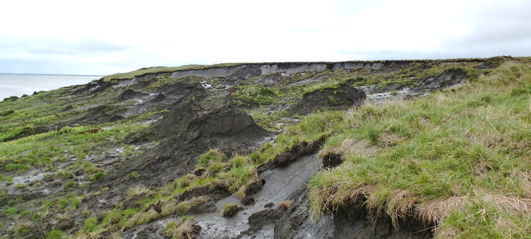
With satellite imagery, we can easily get observations of the entire Arctic. While permafrost itself is mostly subsurface, we can monitor surface indicators closely linked to permafrost health or degradation. One such example are retrogressive thaw slumps (RTS), slow landslides resulting from the thawing of ice-rich permafrost. Despite their small size and scattered distribution, RTS can be detected in satellite images due to their distinct shape and spectral signature.
But here’s the catch: While deep learning algorithms show promise in identifying RTS from satellite images, they need huge amounts of labeled training data. In fact, only a very small fraction of the Arctic has been labelled for RTS:
Available footprints of RTS in the Arctic. Pick a site in the drop-down menu to zoom in on that region on interest.
Acquiring labelled data is no easy feat, as permafrost experts need to manually look through large satellite imagery archives and label examples pixel-by-pixel. Clearly, it is impossible to cover large fractions of the Arctic in this way. So ideally, we are looking for ways to get our models to generalize to new locations without the need for extensive labeled data. Therefore, we are exploring a new way of enhancing this generalisation ability without additional labels in our recent study.
What is DINO?
In an ideal setup, we can not only use the existing labelled data, but also teach the model to extract knowledge from unlabelled imagery of previously unseen regions. This hybrid setup is known as semi-supervised learning.
DINO is a method for training AI models without any labelled examples. Instead of relying on human-labeled data, it lets the computer figure out its own way to recognize objects in pictures and classify them. Intuitively, it gives the network the following rules:
- Assign a class label to each training image
- Make sure that the class labels remain the same when the image is transformed
- Make use of all available labels (given a predefined number of them)
To do this, the DINO learning process introduces two key players: the student and the teacher. They work together to learn from images through a process called self-distillation, making sure to obey the rules stated above. The teacher starts by guessing what’s in an image, then the student tries to match those guesses while also learning from the image itself. It’s like a teacher guiding a student, but in this case, both of them are AI models learning together.
The transformations introduced by the second rule are called Data Augmentations. By randomly applying operations to the input images, we can change the layout (flips, rotations, etc.) or adjust the image colours (brightness, contrast, …). During training, student and teacher will both see differently augmented versions of the same image. The student is then trained to match the teacher’s label.
Visualization of spatial and colourspace augmentations on a Sentinel-2 satellite image from Banks Island, Canada.
That leaves us with the last rule, making the models to use of all of the available classes. For this, DINO introduces two operations, called centering and temperature scaling. So how do these work? When we give it an image, the teacher doesn’t simply predict a single label, but actually gives us a distribution over the class labels. For the centering step, we reduce the weight of frequently used classes, and boost the classes that are less often used. This is done by keeping track of past teacher outputs. For the temperature scaling step, the teacher outputs are adjusted in a way that emphasizes the differences present in the prediction – high-weight classes are given even higher weight, and low-weight classes are tuned down:
Centering and scaling of the teacher output, encouraging use of all classes while deciding for a single class per image.
From DINO to PixelDINO
In the regular DINO scheme, only a single label is assigned to the entire image. But for mapping tasks in remote sensing, we need a class label for each individual location in the image instead. This is what we do with our PixelDINO framework. Instead of classifying whole images, it assigns labels to each pixel in the picture.
A fundamental assumption of DINO training is that augmentations don’t change the class of the image. When working on the pixel level, this is no longer true! When mirroring or rotating an image, the objects within the image change their locations. So not only do we need to augment the imagery for the student, but we also need to transform the teacher labels alongside with it. For this, we take inspiration from another semi-supervised training method, called FixMatchSeg.
Instead of creating two random augmentations of an image, FixMatchSeg builds on a chain of augmentations. A first set, called weak augmentations is applied before passing an image to the teacher. After getting teacher labels for this version of the image, the weakly augmented image is then augmented together with the teacher labels using a second set of augmentations, called strong augmentations. The student then trains to match the teacher’s output on the strongly augmented version of the image.
Overview of the PixelDINO training pipeline used to train a model on unlabelled images.
One final question in this setup is how to learn the teacher’s weights. For this, we adapt the simple, yet effective strategy used by DINO: the teacher follows the student with an exponential moving average. In this way, the teacher is not static, and is updated with newly distilled knowledge.
From self-supervised to semi-supervised
The next step is combining this self-supervised training method with regular supervised training. After all, we do have imagery with existing ground truth annotations, as we saw above. Due to the fact that PixelDINO already works with pseudoclasses, this is very easy! All we need to do is align one of the pseudoclasses with the RTS class that we have given in the training data.
All in all, we arrive at the following training procedure for a single batch (in Pytorch-Pseudocode):
def train_step(img, mask, unlabelled):
  # Supervised Training Step
  pred = student(img)
  loss_supervised = cross_entropy(pred, mask)

  # Get pseudo-classes from teacher
  view_1 = augment_weak(unlabelled)
  mask_1 = teacher(mask_1)
  mask_1 = (mask_1 - center) / temp
  batch_center = center.mean(dim=[0, 2, 3])
  mask_1 = softmax(mask_1)

  # Strongly augment image and label together
  view_2, mask_2 = augment_strong(view_1, mask_1)

  pred_2 = student(view_2)
  loss_dino = cross_entropy(pred_2, mask_2)

  loss = loss_supervised + beta*loss_dino
  loss.backward()  # Back-propagate losses
  update(student)  # Adam weight update
  ema_update(teacher, student)  # Teacher EMA
  ema_update(center, batch_center)  # Center EMA
Results
To evaluate how well our method works, we trained multiple models with different configurations to see how well they classify permafrost disturbances. To make the training process as fair as possible, we counted the number of training steps each model went through instead of using epochs, since our labeled data was much smaller than the unlabeled data. We set aside two regions for testing the models: Herschel Island because it’s an island isolated from the mainland and Lena because it is in a different land cover zone. This helps with seeing how well the models can handle areas they’ve never seen before. We then compared the performance of these models with different configurations to see which training methods worked best.
| Model | Herschel | Lena |
|---|---|---|
| Baseline | 19.8 ± 1.7 | 28.8 ± 3.0 |
| Baseline+Aug | 22.9 ± 3.0 | 25.8 ± 10.2 |
| FixMatchSeg | 23.4 ± 0.8 | 32.4 ± 3.2 |
| Adversarial | 26.6 ± 3.9 | 25.1 ± 15.1 |
| PixelDINO | 30.2 ± 2.7 | 39.5 ± 6.5 |
IoU values achieved by the different models on the Herschel and Lena test regions.
Indeed, PixelDINO outperforms not only the supervised base methods, but also the two other semi-supervised segmentation methods we tested: FixMatchSeg and Adversarial Semi-Segmentation. In practice, this improved training method leads to less false positives and more faithful reconstruction of RTS shapes:
Ground truth and model predictions for a test region near the Lena River (Siberia). PixelDINO greatly reduces false positives compared to a supervised baseline.
The developed PixelDINO method should prove useful not only for permafrost monitoring, but also for other usecases in remote sensing, where spatial variability poses a challenge. We hope that this work can inspire follow-up research for other applications.